Exponential function and Euler's formula without power series
$\newcommand\R{\mathbb{R}}\newcommand\C{\mathbb{C}}\newcommand\Z{\mathbb{Z}}$
Acknowledgements. This was provoked by a Quanta Magazine article by Steven Strogatz on how to prove Euler's formula using power series. The discussion below was inspired by Michael Hutchings' observation that Euler's formula can be proved by solving an ordinary differential equation. I'd also like to thank Dan Lee, Keith Conrad, and my other Facebook friends for their comments and corrections.
Introduction
Euler's formula states that given any real number $\theta$, $$e^{i\theta} = \cos\theta + i\sin\theta.$$ At first, even the meaning of the left side is unclear. The standard approach is to use power series to define $e^{i\theta}$ and prove Euler's formula. The argument is outlined below. It is simple and elegant. I have, however, always found it unsatisfying, since it provides little intuition into what's going on.
Here, I provide an alternative approach that I find that is easier to understand intuitively.. Moreover, it accomplishes much more. From nothing more than elementary calculus (and some elementary real analysis if you want rigorous proofs), it provides definitions of the constants $\pi$ and $e$, as well as definitions and basic properties of the exponential, sine, and cosine functions, including Euler's formula.
Power series proof of Euler’s formula
Here is a brief outline of how to prove Euler's formula using power series. The starting point are the power series \begin{align} e^{x} &= \sum_{k=0}^\infty \frac{x^k}{k!} = 1 + x + \frac{x^2}{2!} +\cdots \label{taylor}\\ \sin x &= \sum_{k=0}^\infty (-1)^k\frac{x^{2k+1}}{(2k+1)!} = x - \frac{x^3}{3!} + \frac{x^5}{5!} + \cdots \notag\\ \cos x &= \sum_{k=0}^\infty (-1)^k\frac{x^{2k}}{(2k)!} = 1 - \frac{x^2}{2!} + \frac{x^4}{4!} + \cdots. \notag \end{align} It follows by the ratio test that these series converge for every $x \in \R$. The key observation is that these power series also converge if $x$ is complex, extending the domains of these functions from $\R$ to $\C$. Euler's formula now follows by setting $x = i\theta$ in \eqref{taylor} and splitting the series into its real and imaginary parts, \begin{align*} e^{i\theta} &= \sum_{k=0} \frac{(i\theta)^k}{k!}\\ &= \sum_{k=0} (-1)^k \frac{\theta^{2k}}{(2k)!} + i\sum_{k=0} (-1)^k \frac{\theta^{2k+1}}{(2k+1)!}\\ &= \cos\theta + i\sin\theta. \end{align*} This is simple and elegant, but the proof provides little intuition to what is going on. Euler's formula appears magically.
Below is an alternative approach that I think elucidates how the exponential function of both real and imaginary numbers arise and why exponential of an imaginary number has a geometric interpretation. The explanation below requires only basic calculus. A rigorous discussion requires knowledge of basic real analysis, as presentsed in, say, Abbott's Understanding Analysis.
Exponential of a real number
We start by postulating what we mean by an exponential function of a real number. A function $$ E: \R \rightarrow \R $$ is said to be growing or decaying exponentially if its derivative is proportional to itself. In other words, it is differentiable and, for some real constant $k$, satisfies the equation \begin{equation} E' = kE. \label{ode}\end{equation} An important property of this equation is called translation invariance. This says that if $E: \R \rightarrow \R$ is a solution to \eqref{ode} and $s \in \R$, the function $E_s$ given by \[ E_s(t) = E(s+t) \] is also a solution to \eqref{ode}. This property is exploited, both explicitly and implicitly, extensively below.
Theorem A in the appendix implies the following:
Theorem. Given any $k, e_0 \in \R$, there exists a unique differentiable function $e$ satisfying \begin{equation} E' = kE\text{ and }E(0) = e_0. \end{equation} Moreover $E$ is in fact smooth, i.e., it has derivatives of all orders.
We want, however, to restrict to functions that satisfy $E(0)=1$. For each $k \in \R$, let $e_k: \R \rightarrow \R$ denote the unique function that satisfies $$ e_k' = ke_k\text{ and }e_k(0) = 1.$$ It is straightforward, using the theorem above, to show that for any $s, t \in \R$, \begin{align*} e_k(s+t) &= e_k(s)e_k(t). \end{align*} This in turn implies that, if we define $$ e = e_1(1),$$ then for any rational number $\frac{n}{d}$, $$ e_1\left(\frac{n}{d}\right) = e^{\frac{n}{d}}. $$ These are the exact properties we would expect from an exponential function and justify writing, for any $t \in \R$, $$e_1(t) = e^t.$$
Exponential of an imaginary number
We now turn to the exponential function of a pure imaginary number. At first sight, this is problematic, because $$ e_1(i\theta) $$ cannot be defined by solving \eqref{ode}, because $t$ would have to be complex. The crucial observation is that, in the real case, the theorem above and the chain rule imply that $$ e^{kt} = e_1(kt) = e_k(t). $$ So the trick is to solve for a function $e_i$ satisfying \begin{equation} e_i' = ie_i\text{ and }e_i(0) = 1. \label{ode2} \end{equation} By Theorem A in the appendix, there is a unique solution. This also has the property that $$ e_i(\theta_1 + \theta_2) = e_i(\theta_1)e_i(\theta_2), $$ which justifies writing, for any $\theta \in \R$, $$ e_i(\theta) = e^{i\theta}. $$
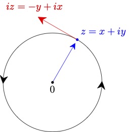
We now want to understand this function better. If we write $e_i(t) = x(t) + iy(t)$, then \eqref{ode2} is equivalent to the system \begin{align*} (x',y') &= (-y,x)\text{ and }(x(0),y(0)) = (1,0). \end{align*} A solution to this satisfies $$ (x',y')\cdot (x,y) = x'x + y'y = -yx + xy = 0 $$ and therefore is a parameterized curve whose velocity vector $$ v = (x', y') $$ is always orthoronal to the position vector $(x,y)$. It also follows easily that \begin{align*} x^2 + y^2 &= 1\\ (x')^2+(y')^2 &= 1. \end{align*} Putting this all together, we see that the solution is a unit speed parameterization of the circle.
It is shown in the appendix that there exists $T > 0$ such that $$ z(T) = z(0). $$ The translation invariance of \eqref{ode2} implies that $z$ is in fact periodic and, for any $\theta \in \R$, $$ z(\theta + T) = z(\theta). $$ We can now define the constant $\pi$ by $$ T = 2\pi. $$ and the functions \begin{align*} \cos\theta &= x(\theta)\\ \sin\theta &= y(\theta). \end{align*} Direct consequences include $$ (\sin\theta)^2 + (\cos\theta)^2 = 1, $$ Euler's formula $$ e^{i\theta} = \cos\theta + i\sin\theta, $$ and \begin{align*} \frac{d}{d\theta}(\sin\theta) &= \cos\theta\\ \frac{d}{d\theta}(\cos\theta) &= -\sin\theta. \end{align*} It is also straightforward to use the symmetries of \eqref{ode2} to derive all of the basic properties of the sine and cosine functions, such as: \begin{align*} \sin(n\pi) &= 0\\ \sin\left(\frac{\pi}{2}+2\pi n\right) &= 1\\ \sin\left(\frac{3\pi}{2}+2\pi n\right) &= -1\\ \cos(2n\pi) &= 1\\ \cos((2n+1)\pi) &= -1\\ \cos\left(\frac{\pi}{2}+n\pi\right) &= 0, \end{align*} where $n$ is any integer. Many trigonometric identities also follow easily by raising $e^{i\theta}$ to integer and rational powers.
Exponential of a complex number
Finally, it is now obvious how to define the exponential of a complex number $z$, namely $$ e^{z} = e_z(1), $$ where $e_z$ is the unique solution to the ODE \begin{equation}\label{ode3} e_z' = ze_z\text{ and }e_z(0) = 1. \end{equation} Again, it is straightforward to show that $$ e^{z_1+z_2} = e^{z_1}e^{z_2} $$ and, in particular, $$ e^{x+iy} = e^xe^{iy}. $$
Summary
We have succeeded in using only basic calculus and basic real analysis to obtain the following in a natural and intuitive way:
- Definitions of the constants $e$ and $\pi$
- Definitions and fundamental properties of the functions $e^z$, $\sin\theta$, $\cos\theta$
- In particular, Euler's formula
Appendix
Convergence of continuous functions on a compact interval
Given a compact interval $I \subset \R$, let $C(I)$ denote the space of continuous complex-valued functions with domain $I$. Given $f \in C(I)$, denote the sup norm of $f$ by \(\|f\| = \sup_{x \in I} |f(x)|.\)
A sequence $f_0, f_1, \dots \in C(I)$ is a Cauchy sequence if for any $\epsilon > 0$, there exists $N>0$ such that for any $j, k \ge N$, \[ \|f_j-f_k\| \le \epsilon. \]
The following is a standard result in basic real analysis (see, for example, Theorems 4.4.7 and 6.2.6 in the book Understanding Analysis by Abbott.
Lemma 1 Given a compact interval $I$, any Cauchy sequence $f_0, f_1, \dots \in C(I)$ converges to a limit $f \in C(I)$.
Contraction map
A map $\Phi: C(I) \rightarrow C(I)$ is a contraction mapping if there exists $c < 1$ such thatfor any $f_1, f_2 \in C(I)$, \[ \|\Phi(f_)) - \Phi(f_2)\| \le c \|f_1-f_2\|. \]
Lemma 2. If $\Phi: C(I) \rightarrow C(I)$ is a contraction map, then there exists a unique $f \in C(I)$ satisfying \begin{equation}\label{fixed} \Phi(f) = f. \end{equation}
Proof. Let $f_0 = 0$ and for each $k \ge 0$, let \[ f_{k+1} = \Phi(f_k). \] First, for any $i > 0$, \begin{align*} \|f_{i+1}-f_{i}\| &= \|\Phi(f_{i})-\Phi(f_{i-1})\|\\ & \le c\|f_{i}-f_{i-1}\|\\ \dots &= c^i\|f_1-f_0\|. \end{align*} Therefore, for any $j, k > 0$, \begin{align*} \|f_k-f_j\| &= \left\|\sum_{i=j}^{i=k-1} f_{i+1} - f_{i}\right\|\\ &\le \sum_{i=j}^{i=k-1} \|f_{i+1} - f_i\|\\ &\le \sum_{i=j}^{i=k-1} c^i\|f_1-f_0\|\\ &= \frac{c^j}{1-c}\|f_1-f_0\|. \end{align*} For any $\epsilon > 0$, if $N$ satisfies \[ \frac{c^N}{1-c} \le \epsilon, \] then for any $j, k \ge N$, \[ \|f_k-f_j\| \le \epsilon. \] It follows that the sequence $f_0, f_1, \dots$ is a Cauchy sequence and therefore, by Lemma 1, has a limit $f \in C(I)$. Moreover, $\Phi(f_0), \Phi(f_1), \dots$ is also a Cauchy sequence. Therefore, \begin{align*} f &= \lim_{k\rightarrow\infty} f_{k+1}\\ &= \lim_{k\rightarrow\infty} \Phi(f_k)\\ &= \Phi(f), \end{align*} which shows that $f$ satisfies \eqref{fixed}. If $f_1, f_2$ both satisfy \eqref{fixed}, then \begin{align*} \|f_1-f_2\| &= \|\Phi(f_1)-\Phi(f_2)\|\\ &\le c\|f_1-f_2\|, \end{align*} which implies that \[ (1-c)\|f_1-f_2\| = 0. \] This proves the uniqueness of the solution.
Existence and uniqueness of solution to \eqref{ode3}
Theorem A. Given $e_0, z \in \C$, there exists a unique differentiable function $e: \R \rightarrow \C$ satisfying \begin{equation}\label{ivp} e' = ze\text{ and }e(0) = e_0. \end{equation}
Proof. Fix $T \in \R$, $\delta > 0$, and $e_T \in \R$. If $e \in C^1([T-\delta,T+\delta])$ satisfies \begin{equation}\label{ivp2} e' = ze\text{ and }e(T) = e_T \end{equation} then, by the fundamental theorem of calculus, \begin{equation}\label{integral-equation} e(t) = e_0 + z\int_{\tau=T-\delta}^{\tau=t} e(\tau)\,d\tau. \end{equation} Let $\Phi: C([T-\delta,T+\delta]) \rightarrow C([T-\delta,T+\delta])$ be given by \[ \Phi(f)(t) = e_T + \int_{\tau=T}^{\tau=t} f(\tau)\,d\tau. \] Then \begin{align*} \|\Phi(f_1)-\Phi(f_2)\| &\le |z|\left\|z\int_{\tau=T}^{\tau=T+\delta} |f_1(\tau)-f_2(\tau)|\,d\tau\right\|\\ &\le |z|\delta\|f_1-\|f_2\|. \end{align*} Therefore, if \[ |z|\delta < 1, \] then $\Phi$ is a contraction map and therefore, there is a unique solution $e \in C([T-\delta,T+\delta])$ to \eqref{integral-equation}. Observe that the equation implies that if $e \in C([T-\delta,T+\delta])$, then $e \in C^1([T-\delta,T+\delta])$. Differentiating \eqref{integral-equation} yields \eqref{ivp}. Observe that in fact $e \in C^\infty([T-\delta,T+\delta])$.
We now want to prove the existence of a solution on $\R$. For each $k \in \Z$, let \[ T_k = \frac{k\delta}{2} \] and \[ I_k = [T_k-\delta,T_k+\delta] = \left[\frac{(k-2)\delta}{2}, \frac{(k+2)\delta}{2}\right]. \] Observe that \[ I_{k}\cap I_{k+1} = \left[\frac{(k-2)\delta}{2}, \frac{(k+2)\delta}{2}\right] \cap \left[\frac{(k-1)\delta}{2}, \frac{(k+3)\delta}{2}\right] = \left[\frac{(k-1)\delta}{2}, \frac{(k+2)\delta}{2}\right] \] and therefore \[ T_{k-1} = \frac{(k-1)\delta}{2} \in I_{k-1}\cap I_k\text{ and } T_{k+1} = \frac{(k+1)\delta}{2} \in I_k\cap I_{k+1}, \] It follows that any solution $e \in C(I_k\cup\cdots I_0 \cup \cdots I_k)$ extends uniquely to a solution $e \in C(I_{k-1}\cup \cdots I0 \cdots \cup I_{k+1})$. By induction, it follows that there exists a unique solution to \eqref{ivp}